
Machine learning based optimization method for vacuum carburizing process and its application
 0
0Abstract
This paper develops an optimized prediction method based on machine learning for optimal process parameters for vacuum carburizing. The critical point is data expansion through machine learning based on a few parameters and data, which leads to optimizing parameters for vacuum carburization in heat treatment. This method extends the data volume by constructing a neural network with data augmentation in the presence of small data samples. In this paper, the database of 213 data is expanded to a database of 2,116,800 data by optimizing the prediction. Finally, we found the optimal vacuum carburizing process parameters through the vast database. The relative error of the three targets is less than that of the target obtained by the simulation of the corresponding parameters. The relative error is less than 5.6%, 1%, and 0.02%, respectively. Compared to simulations and actual experiments, the optimized prediction method in this paper saves much computational time. It provides a large amount of referable process parameter data while ensuring a certain level of accuracy.
Keywords
INTRODUCTION
Various heat treatment techniques, including hardening, carburizing, and tempering, are often used in material processing to provide critical components for aerospace, high-speed railroads, and automobiles with sufficient high strength and high resistance to friction and wear. However, deformation in the heat treatment process has been challenging to predict and control[1- 2]. In particular, the usual carburizing and hardening processes often result in significant and irregular deformations, making it difficult to predict how much machining allowance to leave for subsequent machining of these critical parts and creating difficulties in ensuring high performance and accuracy of the details. Recently, vacuum carburizing and quenching technology have been developed to solve this problem. In particular, the gas quenching method is adopted after vacuum carburization. This method can significantly reduce the deformation caused by quenching and play a good role in improving the performance and precision of parts[3]. However, controlling a vacuum carburizing furnace is more complicated than the standard carburizing technology. It is still basically through many experimental methods to seek to meet the requirements of various materials and parts shapes and performance of the vacuum carburizing process. Therefore, efficiently finding out the best approach to vacuum carburizing and quenching is essential in vacuum carburizing technology.
In vacuum carburizing, steel parts are heated under a vacuum, a "carburizing phase" in which hydrocarbon gases are introduced at low pressure and held in a vacuum to allow the carbon to diffuse into the steel, and this "diffusion phase" results in a uniform hardness of the carburized layer and reduced part deformation[4]. The process of vacuum carburizing is outlined as follows: The carburizing furnace is heated to the required temperature for carburizing under a particular heating process, kept stable, and then forced carburizing and diffusion are performed sequentially. After the diffusion time, reduces the furnace temperature. However, conditions such as heating temperature and carburization time in a vacuum, diffusion temperature and time, as well as gas pressure, have a significant influence on the concentration and depth of the carburized layer on the surface of the carburized part and should be optimally determined according to the steel properties and the part application[5].
As early as 1992, some scholars proposed a thermal-phase-change-mechanical theory and simulation method for heat treatment simulation[6-9], and this theory and calculation method have been used to simulate and verify the heat treatment process of many typical parts. Mechanisms and computational methods that consider the diffusion of carbon inside the steel during carburization have also been proposed and experimentally verified before[10]. Recently, with the development of vacuum carburizing technology, the simulation method has also received attention and research[11].
The simulation technique can indeed describe the changes in the temperature field, diffusion field, phase change, and stress-strain field during heat treatment and reveal the relationship and mechanism of multi-field coupling. However, finding the best process in the heat treatment process is still tough. Although a large amount of data can be obtained through many simulations such as software, the calculations take much time and work to get the process parameters from the target values. To solve this topic, with the development of artificial intelligence techniques, neural networks, and machine learning techniques, machine learning methods have started to find the optimal process for carburizing and quenching[12]. In this paper, we also use neural networks and machine learning methods to propose a linear regression of trained teacher signals and expand the set of teacher signals for a small sample multi-objective vacuum carburization process. The vacuum carburizing process controls and reduces essential parts' thermal deformation and improves surface hardness. It has also received increasing attention in the heat treatment of crucial components such as gears and bearings. It is currently a more effective technology for energy conservation and emission reduction in heat treatment. However, what kind of vacuum carburizing process should be adopted for various shapes and materials to achieve the best effect has always been an urgent issue in applications. In the past, it was predicted through multiple heat treatment simulations to determine the carbon concentration, phase transformation, structure, and hardness changes within parts after vacuum carburizing. Although this simulation has a solid theoretical background, it requires long calculation times and often requires many iterations to find the best process conditions. This paper uses a heat treatment simulation to establish a small sample of teacher signal sets. Through neural networks and machine learning models, it optimizes the design of the vacuum carburizing process. This not only improves the efficiency of process optimization but, more importantly, proposes an efficient and low-cost solution for the process design of vacuum carburizing by combining heat treatment simulation with deep learning technology. Compared with the previous research[13], the innovation of this paper is that the vacuum carburizing data of small samples can be expanded according to the corresponding physical laws within a specific range of error, and the derivation from the demand target to the optimal process parameters can be completed. After the continuous expansion of the data set and deep learning, we find the vacuum carburizing process parameters closest to the target values of carburizing layer depth, surface carbon concentration, and hardness. At the same time, the obtained optimized process parameters are then validated by simulation, and the validation results are confirmed to be superior to the initially empirically adopted process parameters, thus verifying the reliability of the small-sample multi-objective optimization search method proposed in this paper.
SUMMARY OF THE THEORETICAL MODEL
The carburizing and quenching process allows the phase transformation structure of the material to be changed. Mechanical components, such as gears, bearings, and rollers, which place high demands on the surface in terms of resistance to friction and wear, can be substantially hardened and improved by the carburizing process. However, the carburizing and quenching involves a complex continuous medium thermodynamic theory. It requires considering the coupling between the carbon concentration diffusion field, temperature field, phase transformation kinetics, tissue distribution, and the inelastic stress/strain field. In this theory, the coupling effects of the following aspects are considered. The first is carefully considering the impact on material properties and phase transformation kinetics due to the diffusion of carbon ions in the steel and the creation of a gradient distribution. The second considers the effect of temperature changes on the nucleation and growth of phase distortion and the temperature field due to the generation of latent heat from the phase transformation. The development of the phase transformation affects the stress and strain fields as the phase transformation brings about local expansion or contraction.
Conversely, the stress/strain fields can also inhibit or induce the nucleation and growth of the phase transformation. The third aspect is that changes in the temperature field inevitably lead to the expansion or contraction of the material, i.e., thermal strain. When significant distortions occur within the material because of processing and heat treatment, heat generation also occurs, affecting the temperature field change. This is the phenomenon of multi-field coupling in the heat treatment process. Heat treatment simulation software (e.g., COSMAP - Computer Simulation of Manufacturing Process) has been used to simulate the coupled diffusion analysis, temperature analysis, phase transformation, and deformation/stress distribution during carburizing and quenching processes[13].
COSMAP simulation calculations have been validated many times and are consistent with the corresponding physical laws. Therefore, the data obtained from COSMAP simulations can be used as a teacher signal for vacuum carburizing optimization. However, calculations must be made using a large amount of data and time to determine the optimum conditions for the carburizing process. This needs to fit the immediate development needs of new energy vehicles. In developing new energy vehicles, the precision and time required for carburizing and quenching automobile parts are relatively high. Optimization or artificial intelligence technology is expected to propose a method to predict the optimal vacuum carburizing process conditions.
Figure 1 shows the basic theoretical diagram of COSMAP. Analysis code is built with multi-solvers for direct and ICCG methods, allowing a flexible choice of analysis method depending on the analysis problem FEMAP or GiD is used as GUI. It also supports a heat transfer coefficient identification program and a material database interface. It allows the following analysis systems to be constructed: -A material database for the analysis of the material database. The material database is MATEQ, developed by the Material Database Study Group of the Plasticity Engineering Division Committee of the Society of Materials Science, Japan. The user's identification program should be used to identify heat transfer coefficients. Currently, most of the teacher signals in this paper are derived from COSMAP simulation data; the COSMAP simulation data will also be optimized and adjusted for accuracy based on experimental data.
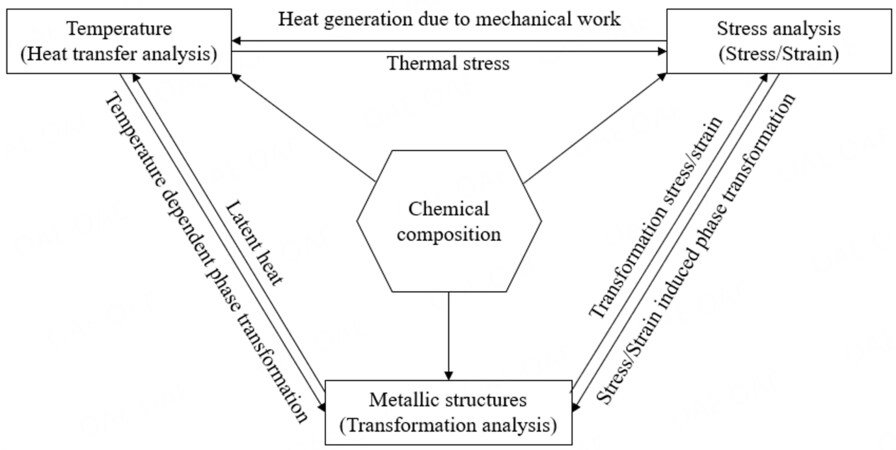
Figure 1. Basic theoretical diagram.
Based on the basic principles of heat treatment and COSMAP, a virtual heat treatment system (VHT) is proposed. The diagram of the heat treatment virtual manufacturing system is shown in Figure 2.
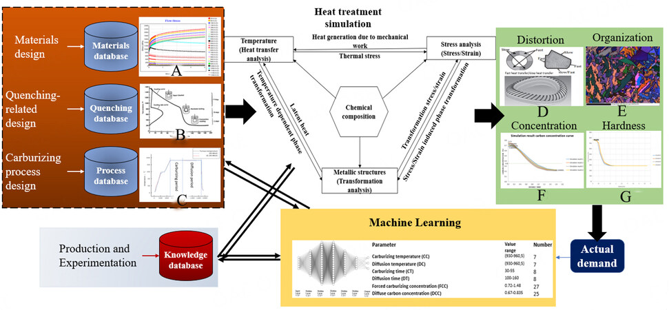
Figure 2. Overview of the heat treatment optimization process; A: Stress-strain analysis of materials; B: Quenching process; C: Vacuum Carburizing Process; D: Gear deformation; E: Part organization diagram; F:carbon concentration distribution; G: Hardness distribution.
Figure 2 shows an overview of the current virtual heat treatment system, including the optimization process. First, the material, quenching, and process databases are constructed using material design, quenching-cooling, and carburizing process designs. We have established the carburizing and quenching knowledge base according to the actual production and experimental results. In this database, this paper can obtain about 30 groups of vacuum carburizing experimental data of cylinders with different materials and use the materials represented by six data groups for research. From the data of these four databases, heat treatment simulations are performed to obtain characteristics regarding deformation, organization, carbon concentration distribution, and hardness distribution. However, the data characteristics are small, and the simulation and calculation could be more convenient. Therefore, 213 sets obtained from simulation and three experimental data sets are used as training data sets. The amount of data is expanded by machine learning to improve the speed of receiving process parameters from the demand, cross-checking with the database before putting them into the actual market, and finally responding to honest requests. To determine the optimum conditions for the carburizing process, many simulation calculations and experiments sometimes lead to a different solution. Methods to predict the optimum vacuum carburizing process conditions need to be proposed. Generate more vacuum carburizing process parameters through learning and training based on small sample data.
This paper presents a method of process optimization based on machine learning and heat treatment simulation techniques and performance characteristics in the context of a specific database size with material-related information already available, which ultimately serves the heat treatment simulation system. Firstly, some of the vacuum carburization simulation data required for the study was used as the initial database. Secondly, the neural network structure is established and trained, and results are tested based on the total number of samples in the database and the target number. If the test results are poor or do not meet the criteria, the neural network is retrained by modifying it or the number of training sessions, for example. Then, once the training results pass the test criteria, data is expanded by data augmentation to keep it at a reasonable range and the correct total number. The expanded data is then optimally predicted by the optimization system in this paper to obtain the closest data to the desired target value. The data parameters obtained from the optimization are then simulated, and various comparison methods evaluate the effectiveness of the optimization. When a certain optimization level has been achieved, the final validation is carried out using experimental results. Finally, the validated data can be used as training samples in the database to improve the training results.
RESEARCH THEORY AND EXPERIMENTAL METHODS
In the initial phase of vacuum carburizing, after obtaining the required target values from the customer, a certain quantity of vacuum carburizing process conditions is first listed based on physical laws and experience to form the basis for the initial parameter data. Carburized quenching simulations are then carried out using software such as COSMAP. Suppose the results of the simulation experiments contain results that match the target values. In that case, the parameters for which the target values are obtained are set as the correct process parameter conditions. However, due to changes in the materials used for vacuum carburizing and accuracy requirements, it is almost impossible to obtain accurate data when setting the initial vacuum carburizing process conditions. Therefore, a more reasonable method is to use several vacuum carburizing process conditions, get the corresponding target values for each by carburizing and quenching simulation, and build a new database as a teacher signal. The advantage of the teacher signals conveyed by this method is that they fit the physical logic of carburized quenching and allow a large amount of data to be obtained relatively quickly. The disadvantage is that the data obtained from the simulation has a high degree of accuracy compared to the data from the actual experiment but needs to be fully representative of the existing experimental data. Based on the teacher signals obtained here, the optimization method of this paper yields one or more combinations of process parameters that are compatible with the target values, provided that specific errors are tolerated. The obtained parameters are calculated by carburized quenching simulation. If the error between the simulation results and the target values is within acceptable limits, actual operating experiments are conducted to determine whether these parameters are correct.
The artificial neural network initially used in this paper is a Multilayer Perceptron, and the specific structure is shown in Figure 3. The design of the multilayer perceptron is one input layer, five hidden layers, and one output layer. The number of nodes is 6 * 12 * 20 * 20 * 12 * 6 * 1.
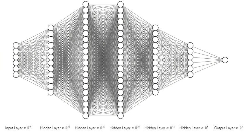
Figure 3. Neural network structure at the beginning of the experiment.
The Value range of training parameters and targets is shown in Table 1. This paper divides the study into two phases: training and extending the database; and optimizing the predictions. In the first phase, the variables are Carburizing temperature (In the following charts, it is slightly written as CC), Diffusion temperature (DC), Carburizing time (CT), Diffusion time (DT), Forced carburizing concentration (FCC)and Diffuse carbon concentration (DCC), and the targets are Carburizing layer depth (CLD), Surface carbon concentration (SC)and Surface hardness (SH). In the second phase, the opposite is true. Throughout the calculations, the carbon concentration, temperature, and phase change tissue volume rate at each node inside the model used, and the stresses and strains are time-dependent process parameters. This paper uses a neural network to solve the linear regression problem instead of a simple linear function. The main reason is that the problem studied in this paper has six feature variables with interactions. In such cases, obtaining suitable linear regression equations separately for each objective is difficult. Training with a neural network can learn feature interactions and increase the model's accuracy. We choose neural networks for data expansion from the following perspectives: the experiments in this paper contain six variables and three target parameters, and the relationship between them is complex, making it difficult to calculate and obtain results using FEM. In terms of physical laws, if a simple linear function is used to fit the relationship between input and output, it will lead to difficulty in regression. The reason for predicting these three parameters is that in vacuum carburizing, they quantify the carburizing effect from different angles, thus determining whether the carburized metal is ready for use. We chose a neural network instead of FEM because the experiment in this paper contains six variable parameters and three interrelated target parameters, and the relationship between them is very complex, so it is not easy to use FEM to calculate and obtain results. FEM simulations can be computationally intensive and require enormous computing resources, especially for complex systems and high-resolution simulations. Machine learning models can be trained using a large amount of data and can be computationally efficient for predicting outcomes once the model is introduced. In the research addressed in this paper, for example, when simulating the target value of vacuum carburization using the corresponding simulation software, the number of model nodes used was 6531, and it took 7 hours for one complete simulation. The data extended by the neural network used in this paper will not fully comply with the fundamental physical laws. Still, it complies with the corresponding laws used in the simulation software calculation, and the computation time is one hour.
Value range of training parameters and targets
| Parameter | Value range | Example |
| Carburizing temperature (CC) (°C) | 930/960 | 930 |
| Diffusion temperature (DC) (°C) | 930/960 | 930 |
| Carburizing time (CT) (min) | (30~55,5) | 35 |
| Diffusion time (DT) (min) | (135~160,5) | 150 |
| Forced carburizing concentration (FCC) (%) | 0.72~0.885 | 0.74 |
| Diffuse carbon concentration (DCC) (%) | 0.67~0.835 | 0.69 |
| Carburizing layer depth (CLD)(mm) | 0.698~1.43 | 0.76886 |
| Surface carbon concentration (SC) (%) | 0.668~0.824 | 0.688 |
| Surface hardness (SH) (HV) | 754.3-783.6 | 764.50897 |
The meaning of (30~55, 5) in the table is to set the value range from 30 to 55 and obtain samples at five intervals. All other identical formats in the table have the same meaning as above. The two brackets after the parameter are the abbreviation and the parameter unit. In this paper, such abbreviations and branches are used after that.
In addition to the above parameters, there are other conditions for vacuum carburizing, such as pressure, material, model construction, and the pulsing process used for carburizing. The model's material and structure are consistent in the simulation using corresponding calculation files; the simulation is carried out at the same pressure (the pressure used in the experiment) by default. Finally, the carburizing concentration parameters are adjusted in the file to match the pulsing process.
To overcome the difficulty of machine learning algorithms to obtain robust prediction results and excellent prediction accuracy with small samples, mega-trend-diffusion (MTD) is used to estimate the acceptable range of attributes for small data sets, to fill the information interval and to calculate the virtual sample value and the affiliation function value (the probability of occurrence of that sample value). This paper uses a multi-distribution mega-trend-diffusion (MD-MTD) technique based on the basic MTD, as shown in Figure 4[14].
Given a sample set X = {x1, x2,...,xn}, the basic MTD estimates the acceptable bounds for X. The lower bound Equation gives l and the upper set U for the excellent range of X.
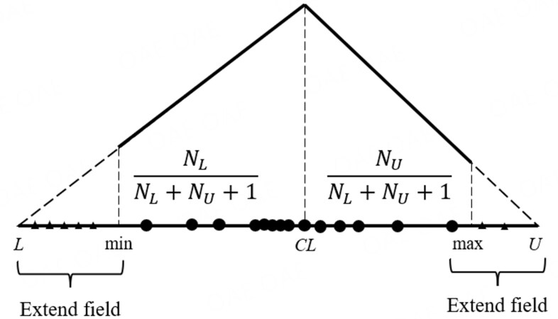
Figure 4. Diagram of MD-MTD.
Among them,
In Equation
n denotes the small sample set size, CL denotes the data center, NU (NU) represents the number of sample values less than (greater than) CL, S2 denotes the small sample set variance, and skewl (skewu) denotes the left (right) skewness describing the non skewl (skewu) denotes the left (right) skewness describing the non-symmetric diffusion characteristics of the data.
The roll-out regions of the sample set X are [L, min] and [max, U], and the directly observed part is [min, max]. Since the data distribution is unknown in the roll-out regions [L, min] and [max, U], a uniform distribution is used to generate virtual sample points, represented as triangular hollow points in Figure 2. In the direct observation region [min, max], the data distribution is described by a triangular distribution, with the closer to the data center CL, the more likely the data is to occur and the more concentrated the data is in the distribution; the further away from the data center CL, the less likely the data is to happen and the more dispersed the data is in the distribution. The virtual sample points in the roll-out area add additional information, and the virtual sample points in the direct observation area fill in the information gap of the original discrete observation points.
Through the MD-MTD process, the original sample set X, in terms of training, effectively increases the sample capacity. The MD-MTD process expands the information of the original sample set X. The MD-MTD process is discussed in the following section.
In this paper, the activation function used for the neural network is the ReLU activation function[15].
Reasons to use ReLU are[16]: 1: Network training can be faster because compared to Sigmoid and tanh, derivatives are easier to obtain, backpropagation constantly updates parameters, and its products are simple in uncomplicated form; 2: The ReLU function is a segmented linear function. Classifying a neural network can be regarded as a multi-stage small linear regression process, effectively improving the classification effect; 3: Prevent gradient loss. Suppose the values are too large or too small. In that case, the derivatives of sigmoid and tanh approach zero, and the phenomenon of ReLU being a non-saturated activation function does not exist; 4: To reduce overfitting, make the mesh sparse, with parts smaller than 0 and values larger than 0.
Parameter normalization is carried out once before the training and expansion data. The normalization method uses the MinmaxScaler method uniformly, with the following Eqation (8):
In model training, the three target values are trained independently and used in the MSE loss function to reduce the mutual influence between the target values. The gradient is adjusted by back-propagation. The loss function is shown in Equation:
L is the mean of the sum of squares of the errors, n is the total number of data, ŷi is the fitted data, and yi is the actual data. The formula for updating the gradient is shown in Equation[17].
∂L/∂w and ∂L/∂b are the gradients of the weights (w) and biases (b), n is the total number of data, xi is the original data, and yi is the data from the model. The Adam optimizer is used in the process of optimizing the model[18]; the Adam update rule is:
Calculate the gradient of the t-time steps.
First, the exponential moving average number of gradients is calculated and m0 is initialized to 0. As in the Momentum algorithm, the gradient dynamics of previous time steps are considered comprehensively.
The β1 coefficient is an exponential decay rate, which controls the weight assignment (moving mass and current gradient). It usually takes a value close to 1. The default value is 0.9.
Figure 5 briefly illustrates the case where the gradient of each time step is accounted for as time accumulates in time steps 1~20.
Second, the exponential moving average number of gradient squares is calculated and v0 is initialized to 0. The β2 factor is the exponential decay rate, which controls the effect of previous gradient squares. as in the RMSProp algorithm, the gradient squares are weighted and averaged. The default is 0.999.
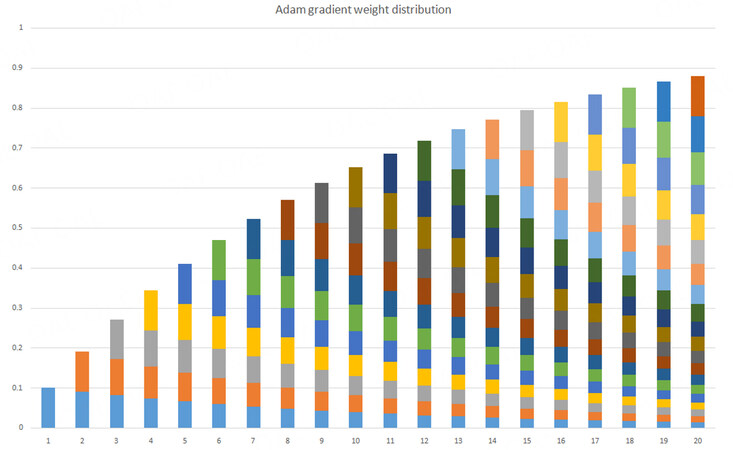
Figure 5. Calculate the gradient for each time step as time accumulates.
Third, since m0 is initialized to 0, mt is biased towards 0, especially in the early training phase. Therefore, a deviation correction should be applied here to the gradient mean mt to reduce the effect of the deviation on the early training phase.
Fourth, when v0 is initialized to 0, the initial training phase vt is biased towards 0 and is therefore modified in the same way as m0.
Fifth, update parameters, multiplying the ratio of the initial learning rate α gradient mean to the square root of the gradient variance. Default learning rate α = 0.001. ε = 10-8, avoiding a divisor of 0. The equation shows that the calculation of updated step length is not directly determined by the current gradient but can be adaptively adjusted from two angles: the gradient means and the gradient square.
The error rates of the three target values are output after each training session to intuitively determine whether the gradient optimization of the current training is standard. The model creation flowchart is shown in Figure 6. First, data are loaded as a teacher signal through the DATA part of the program. After ensuring the data are free of physical and mathematical errors, they are determined and normalized as teacher signals for training the model.
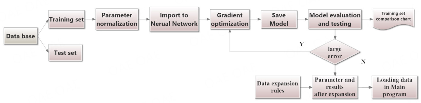
Figure 6. Model Creation Flowchart.
The neural network for the three targets is then introduced through the NET part of the program, introducing three models each; the MSE loss function, Adam optimization algorithm, and error backpropagation are used to optimize the gradients of the models.
After the optimization is completed, the current model is saved. The model is evaluated in the TEST part of the program by the goodness of fit of the data in the test set comparison chart.
If the errors are within acceptable limits, the current model extends the parameter range and generates new data for data loading in the central program part.
TRAINING RESULTS AND DATA EXPANSION
In this paper, to determine how often the training is most appropriate under the current neural network structure, the training results are shown in Figure 7 and Figure 8 for training times 3,500 and training times 5,000, respectively, were tested. See Supplementary Figure 1 and Supplementary Figure 2 for the error rate of training results. The reasons for selecting these two training times are: At the initial research stage, we only set two target values for training, and the neural network is relatively simple. We made 500, 1,000, and 2,000 training attempts during the movement, and finally determined that the results of 1,000 and 2,000 training attempts were similar, and the effect was good. When the target value of the study is increased to 3, the complexity and training difficulty of the neural network will increase significantly because the data rule of the new surface hardness parameter is more complex. In this case, the training result could be better if the training frequency is lower. In addition to the above two training times, we also conducted 7500 and 10000 training times. Most of the time, the training effect is similar to when the number of training is 5000, but it consumes more time, and sometimes there is even greater error.
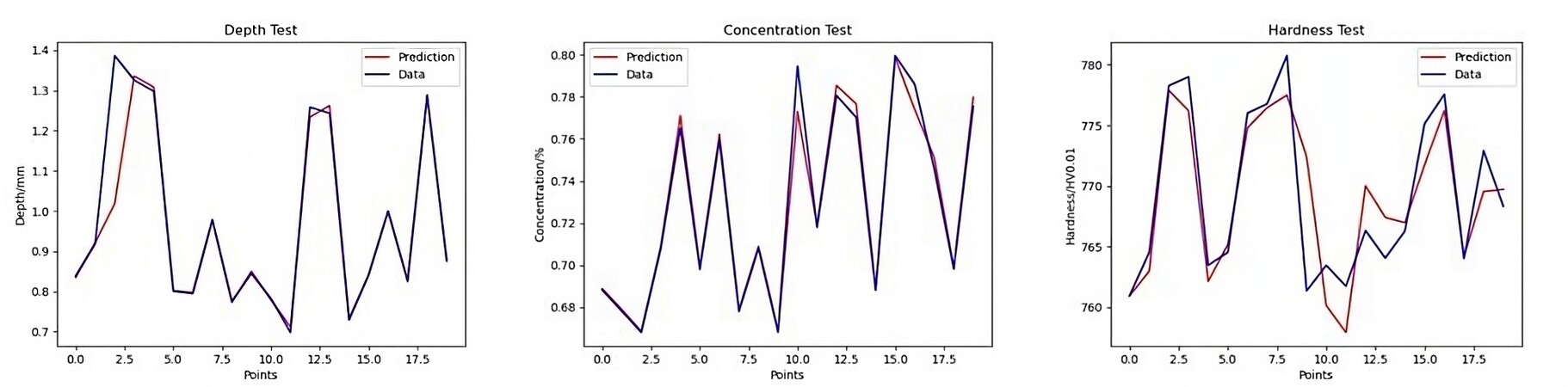
Figure 7. Training results at 3500 training sessions.
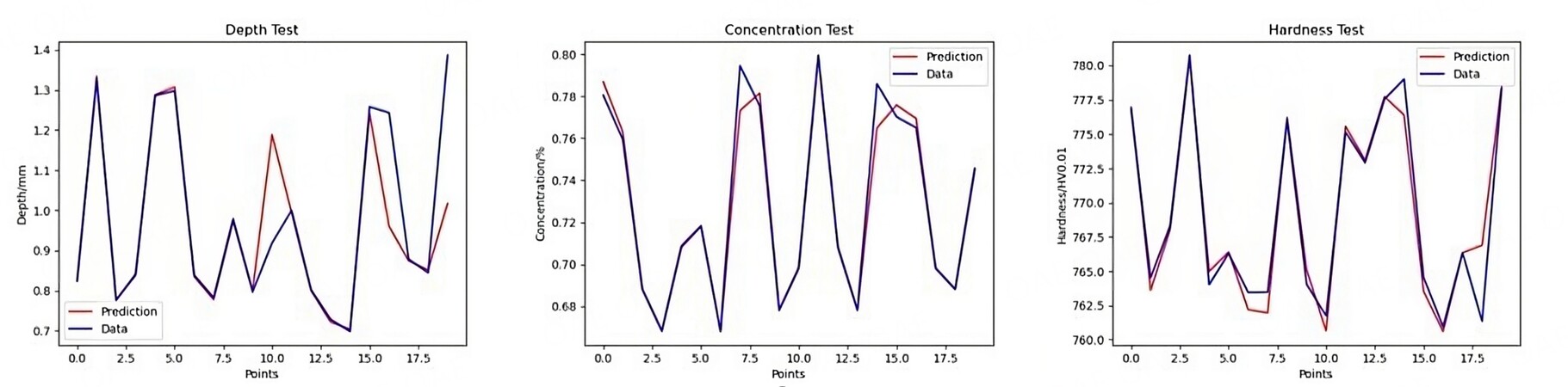
Figure 8. Training results at 5000 training sessions.
We analyze Figure 7 and Figure 8 from the point of view that the test results are consistent with the original data. The coincidence rates of the three target values in Figure 7 are 70%, 60%, and 40%, respectively; The coincidence rates in Figure 8 are 75%, 75%, and 55%. R2 in Figure 7 are 0.987, 0.985, and 0.545. R2 in Figure 8 are 0.928, 0.989, and 0.647. If the training results of carburization layer depth and surface carbon concentration do not differ significantly, the training results of surface hardness are better for a training number of 5,000. Therefore, 5,000 was used as the training number in the subsequent optimization.
The process flow of vacuum carburizing optimization is as follows: First, each process condition is determined, and carburizing and quenching simulations are performed under each process condition using the heat treatment simulation program COSMAP to obtain initial vacuum carburizing process conditions and teacher signals. As the simulated process is theoretically representative of vacuum carburization's physical and chemical phenomena, these teacher signals are introduced into the neural network for learning and training. The appropriate parameter values for each cell in the neural network are determined. On the other hand, if there are few teacher signals, the results obtained in training do not match the demanded target values, so the database must be expanded. However, since the vacuum carburization simulation uses partial differential equations and finite element methods to represent physical and chemical phenomena, expanding the teacher signals by coupled analysis is pretty computationally time-consuming. Therefore, for optimal training, this paper first performs initial training using the initial database (215 pairs) obtained from the simulation, and then the process conditions of vacuum carburization given to the teacher signal are expanded by the rules of linear expansion to including the carburization temperature, diffusion temperature, time interval of each process, and carburization effects (results) are extended, and the training is performed again.
The extension of data is considered based on the following points. 1:The training data contains only two carburizing temperatures, 930°C and 960°C, and the diffusion temperature is the same as the carburizing temperature. Practically all combinations of temperatures between these two temperatures can be obtained based on these two temperatures, and the error is within the range allowed by machine learning; 2:To make the training results more convincing and to make the objective of the data extension clearer, three sets of experimental data with the same material and model as the training data were included in this paper so that the parameters had to be extended to include the corresponding values of the experimental data when the data was developed; 3:Because the data expansion is a complete permutation, each additional parameter value adds a large amount of total data. More total data can seriously affect the speed of data expansion and optimization of predictions. Therefore, we only partially perform the same interval data expansion in this paper. The specific expansion results are shown in Table 2.
Results of data expansion
| Parameter | Value range | Number |
| Carburizing temperature (CC) | (930-960,5) | 7 |
| Diffusion temperature (DC) | (930-960,5) | 7 |
| Carburizing time (CT) | 30-55 | 8 |
| Diffusion time (DT) | 100-160 | 8 |
| Forced carburizing concentration (FCC) | 0.72-1.48 | 27 |
| Diffuse carbon concentration (DCC) | 0.67-0.835 | 25 |
After the range expansion of the parameter values, an array of 6 parameter value ranges is combined to obtain the new database. Therefore, the maximum number of new data is 7*7*8*8*27*25, 2,116,800 pairs. To ensure that the new data generated is reasonable, restrictions are added to the expansion process: the forced carburizing temperature is greater than or equal to the diffusion temperature; and the forced carburizing concentration is greater than the diffusion concentration. The predictions of the process parameters will be determined based on an extended database. Therefore, the experiments will reasonably extend the range of parameter values in the database.
OPTIMIZATION RESULTS FOR PROCESS PARAMETER PREDICTION
This paper uses C# as the front end to call the Python program running on the back end. See Appendix A for the interface of the optimization prediction system. In this optimization result evaluation, the demand target values were set as follows: carburization layer depth 0.95, surface carbon concentration 0.69, and surface hardness 833. One set of experimental data from BMEI is consistent with the currently set requirements; therefore, data relating to a 1/4 cylinder of the same material and size were used in the COSMAP simulations, and the parameters for the simulations were obtained by optimization.
The results of COSMAP simulations are read as shown in Figure 9. The colors and numbers below the hardness and node carbon density indicate the range of values from maximum to minimum values for the corresponding parameters in the graph. The red dotted lines with arrows indicate the position and direction when taking data for the corresponding parameters. The red dotted lines with arrows indicate the position and direction when taking data for the corresponding parameters. The 1/4cylinder model used for the simulation, which has diffusion coefficients designed concerning the full cylinder, can therefore be considered following the same physical laws as the full cylinder due to the symmetry. For the results to follow a consistent reading method with the experimental results, values close to the edges of the cylinder ends were chosen for reading surface hardness and surface carbon concentration. When reading the depth of the carburized layer, the value at 0.35% of the carbon content was read as the depth of the carburized layer. When the graphs in COSMAP do not directly yield specific values for the depth of the carburized layer, the software is used to download the Graph file and form a scatter plot in excel to obtain accurate results. An example of the Graph file transformation is shown in Figure 10.
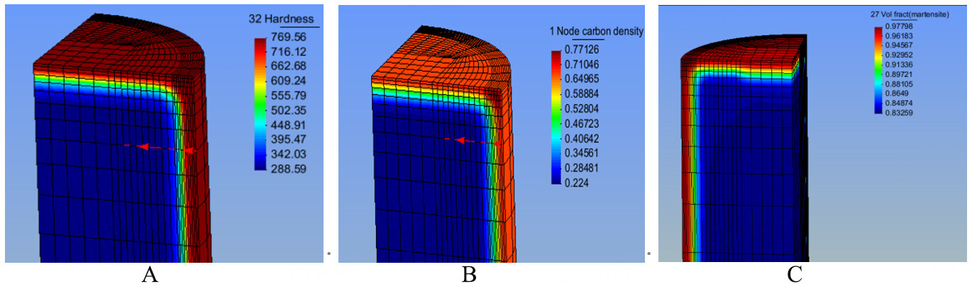
Figure 9. A: Selection of surface hardness; B: surface carbon; C: Martensitic phase transition.
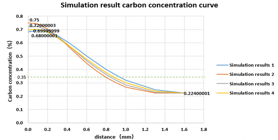
Figure 10. Example of manual image conversion.
The results of the four sets of parameters resulting from the optimization carried out by this system, compared with the target values calculated from simulations with the same parameters, are shown in Table 3.
Relative error of optimization results to simulation results and to experimental data
| Parameter | CC | DC | CT | DT | FCC | DCC | CLD | SC | SH | Description |
| Assumptions | 930 | 930 | 42 | 140 | 1.35 | 0.69 | 0.95 | 0.69 | 833 | Demand |
| Experimental | 930 | 930 | 42 | 140 | 1.35 | 0.69 | 0.95 | 0.69 | 833 | result |
| Optimization1 | 935 | 935 | 49 | 100 | 1.22 | 0.76 | 0.94902 | 0.73557 | 833.0437 | Optimization |
| Result | 935 | 935 | 49 | 100 | 1.22 | 0.76 | 0.103% | 6.604% | 0.005% | Relative error |
| Simulation1 | 935 | 935 | 49 | 100 | 1.22 | 0.76 | 0.75 | 0.76 | 775.47 | Simulation |
| Result | 935 | 935 | 49 | 100 | 1.22 | 0.76 | 21.053% | 10.145% | 6.906% | Relative error |
| Optimization2 | 940 | 940 | 50 | 100 | 1.22 | 0.76 | 0.95795 | 0.743 | 833.0293 | Optimization |
| Result | 940 | 940 | 50 | 100 | 1.22 | 0.76 | 0.837% | 7.681% | 0.004% | Relative error |
| Simulation2 | 940 | 940 | 50 | 100 | 1.22 | 0.76 | 0.707 | 0.76 | 775.51 | Simulation |
| Result | 940 | 940 | 50 | 100 | 1.22 | 0.76 | 15.263% | 10.145% | 6.902% | Relative error |
| Optimization3 | 950 | 950 | 50 | 100 | 1.22 | 0.74 | 0.94334 | 0.73048 | 832.95538 | Optimization |
| Result | 950 | 950 | 50 | 100 | 1.22 | 0.74 | 0.701% | 5.867% | 0.005% | Relative error |
| Simulation3 | 950 | 950 | 50 | 100 | 1.22 | 0.74 | 0.783 | 0.765 | 776.68 | Simulation |
| Result | 950 | 950 | 50 | 100 | 1.22 | 0.74 | 17.579% | 10.870% | 6.761% | Relative error |
| Optimization4 | 950 | 950 | 42 | 100 | 1.26 | 0.765 | 0.97569 | 0.75537 | 832.99841 | Optimization |
| Relative error | 950 | 950 | 42 | 100 | 1.26 | 0.765 | 2.704% | 9.474% | 0.0002% | Relative error |
| Simulation4 | 950 | 950 | 42 | 100 | 1.26 | 0.765 | 0.783 | 0.74 | 773.26 | Simulation |
| Relative error | 950 | 950 | 42 | 100 | 1.26 | 0.765 | 17.579% | 7.246% | 7.172% | Relative error |
The relative errors can be obtained from the three data sets in blue. The relative errors of the target values of the optimization results are smaller than the corresponding simulation results. However, the problem is that the relative error of the surface carbon concentration values in the current case is very large, which theoretically does not play a role in optimization.
For the sake of optimization rigor, the parameters obtained from the optimization are simulated in this paper, and the results are compared with the best results in the original training set. The results are shown in Table 4.
Comparison of optimized parameter simulations with the original optimal data
| Parameter | CC | DC | CT | DT | FCC | DCC | CLD | SC | SH | Description |
| Assumptions | 930 | 930 | 42 | 140 | 1.35 | 0.69 | 0.95 | 0.69 | 833 | Demand |
| Experimental | 930 | 930 | 42 | 140 | 1.35 | 0.69 | 0.95 | 0.69 | 833 | result |
| Simulation1 | 935 | 935 | 49 | 100 | 1.22 | 0.76 | 0.75 | 0.76 | 775.47 | Simulation |
| result | 935 | 935 | 49 | 100 | 1.22 | 0.76 | 21.053% | 10.145% | 6.906% | Relative error |
| Simulation 2 | 940 | 940 | 50 | 100 | 1.22 | 0.76 | 0.707 | 0.76 | 775.51 | Simulation |
| result | 940 | 940 | 50 | 100 | 1.22 | 0.76 | 15.263% | 10.145% | 6.902% | Relative error |
| Simulation 3 | 950 | 950 | 50 | 100 | 1.22 | 0.74 | 0.783 | 0.765 | 776.68 | Simulation |
| result | 950 | 950 | 50 | 100 | 1.22 | 0.74 | 17.579% | 10.870% | 6.761% | Relative error |
| Simulation 4 | 950 | 950 | 42 | 100 | 1.26 | 0.765 | 0.783 | 0.74 | 773.26 | Simulation |
| result | 950 | 950 | 42 | 100 | 1.26 | 0.765 | 17.579% | 7.246% | 7.172% | Relative error |
| Training | 960 | 960 | 40 | 160 | 0.81 | 0.76 | 95.23% | 75.01% | 773.64% | best |
| result | 960 | 960 | 40 | 160 | 0.81 | 0.76 | 0.238% | 8.711% | 7.126% | Relative error |
It is easy to see from the combined error rate that although the optimization results do not achieve the accuracy of the training data in terms of individual target values, they do have an overall optimization effect. However, according to Table 4, the results of the current optimization are smaller than the errors obtained from the original training data when the simulation is re-run, which proves that, in some sense, the recent optimization is not sufficient.
Therefore, in this paper, the structure of the neural network is modified, and a second optimization and simulation calculation is performed. The number of layers of the neural network has changed from 6 to 8, and the maximum number of nodes has increased to 30. Based on the new neural network, training, data expansion, optimization prediction, and simulation calculation are carried out again.
The optimization and simulation results after modifying the neural network with the optimal data of the training set are shown in Tables 5 and 6.
Comparison results of relative errors after modifying the neural network
| Parameter | CC | DC | CT | DT | FCC | DCC | CLD | SC | SH | Description |
| Assumptions | 930 | 930 | 42 | 140 | 1.35 | 0.69 | 0.95 | 0.69 | 833 | Demand |
| Experimental | 930 | 930 | 42 | 140 | 1.35 | 0.69 | 0.95 | 0.69 | 833 | result |
| Optimization1 | 960 | 950 | 50 | 160 | 1.28 | 0.68 | 0.97854 | 0.68676 | 833.12805 | Optimization |
| Result | 960 | 950 | 50 | 160 | 1.28 | 0.68 | 3.00% | 0.47% | 0.0154% | Relative error |
| Simulation1 | 960 | 950 | 50 | 160 | 1.28 | 0.68 | 0.907 | 0.68 | 767.5 | Simulation |
| Result | 960 | 950 | 50 | 160 | 1.28 | 0.68 | 4.526% | 1.449% | 7.863% | Relative error |
| Optimization2 | 960 | 955 | 49 | 120 | 1.26 | 0.72 | 0.96749 | 0.72111 | 832.94519 | Optimization |
| Result | 960 | 955 | 49 | 120 | 1.26 | 0.72 | 1.841% | 4.509% | 0.0066% | Relative error |
| Simulation2 | 960 | 955 | 49 | 120 | 1.26 | 0.72 | 0.865 | 0.7 | 770.19 | Simulation |
| Result | 960 | 955 | 49 | 120 | 1.26 | 0.72 | 8.947% | 1.449% | 7.54% | Relative error |
| Optimization3 | 960 | 960 | 30 | 120 | 1.26 | 0.75 | 0.96773 | 0.74116 | 832.91785 | Optimization |
| Result | 960 | 960 | 30 | 120 | 1.26 | 0.75 | 1.866% | 7.414% | 0.0099% | Relative error |
| Simulation3 | 960 | 960 | 30 | 120 | 1.26 | 0.75 | 0.846 | 0.72 | 773.06 | Simulation |
| Result | 960 | 960 | 30 | 120 | 1.26 | 0.75 | 10.947% | 4.348% | 7.196% | Relative error |
| Optimization4 | 960 | 960 | 35 | 155 | 1.22 | 0.7 | 0.89685 | 0.69691 | 833.00464 | Optimization |
| Result | 960 | 960 | 35 | 155 | 1.22 | 0.7 | 5.60% | 1.00% | 0.0006% | Relative error |
| Simulation4 | 960 | 960 | 35 | 155 | 1.22 | 0.7 | 0.81 | 0.75 | 768 | Simulation |
| Result | 960 | 960 | 35 | 155 | 1.22 | 0.7 | 14.737% | 8.696% | 7.80% | Relative error |
Comparison results of simulated data after modifying the neural network
| Parameter | CC | DC | CT | DT | FCC | DCC | CLD | SC | SH | Description |
| Assumptions | 930 | 930 | 42 | 140 | 1.35 | 0.69 | 0.95 | 0.69 | 833 | Demand |
| Experimental | 930 | 930 | 42 | 140 | 1.35 | 0.69 | 0.95 | 0.69 | 833 | result |
| Simulation 1 | 960 | 950 | 50 | 160 | 1.28 | 0.68 | 0.907 | 0.68 | 767.5 | Simulation |
| result | 960 | 950 | 50 | 160 | 1.28 | 0.68 | 4.526% | 1.449% | 7.863% | Relative error |
| Simulation 2 | 960 | 955 | 49 | 120 | 1.26 | 0.72 | 0.865 | 0.7 | 770.19 | Simulation |
| result | 960 | 955 | 49 | 120 | 1.26 | 0.72 | 8.947% | 1.449% | 7.54% | Relative error |
| Simulation 3 | 960 | 960 | 30 | 120 | 1.26 | 0.75 | 0.846 | 0.72 | 773.06 | Simulation |
| result | 960 | 960 | 30 | 120 | 1.26 | 0.75 | 10.947% | 4.348% | 7.196% | Relative error |
| Simulation 4 | 960 | 960 | 35 | 155 | 1.22 | 0.7 | 0.81 | 0.75 | 768 | Simulation |
| result | 960 | 960 | 35 | 155 | 1.22 | 0.7 | 14.737% | 8.696% | 7.80% | Relative error |
| Training | 960 | 960 | 40 | 160 | 0.81 | 0.76 | 0.95226 | 0.75010598 | 773.64301 | best |
| result | 960 | 960 | 40 | 160 | 0.81 | 0.76 | 0.238% | 8.711% | 7.126% | Relative error |
Although the relative errors of each target value are smaller than the corresponding simulated data for only two sets of data after modifying the neural network, the relative errors of each target value are small enough to achieve the optimization effect. In some cases, substituting the parameters of the optimization results back into the simulation gives results with more minor errors than the training data. The combined error rate also becomes smaller compared to the training data and can justify this method of modifying the neural network.
CONCLUSIONS
In this paper, a machine learning-based optimization method for the vacuum carburizing process is developed. The plan is based on the database provided by the heat treatment simulation and computation system. A multilayer perceptron neural network is used to build a vacuum carburizing optimization prediction system to train and extend the data of vacuum carburizing to obtain more training and optimization parameters with small samples. Currently, the optimization and prediction method proposed in this paper is based on 213 sets, which were expanded to 2,116,800 locations through neural network training and data expansion. The training results were tested with a comparison R2 of 0.928, 0.989, and 0.647 within an acceptable error range. Using the expanded database as a basis for predicting the optimal vacuum carburizing process parameters, the expected parameters for the three objectives had relative errors that were better than the corresponding simulated results, and the relative errors were all maintained below 5.6%, 7.414%, and 0.0154%, respectively. At the beginning of the study, the neural network used was six layers, which was gradually fixed to use a neural network with eight layers. After simulation and calculation, the maximum number of nodes was adjusted from 30 to 32 layers. It was finally possible to make the simulation results of the parameters obtained by the optimized system better than the optimal data in the initial database. Compared with the standard vacuum carburizing process parameters calculation, the method is characterized by the following. 1:Fast analysis and application of the vacuum carburizing simulation data; 2: The process parameter data obtained by optimization can be used as new data for the database within a specific error allowance.
After the data extension is completed, the extended data set is used as a database for process optimization. When numerical requirements are made for the vacuum carburizing process regarding the carburizing layer depth, surface carbon concentration, and hardness, the process parameters with the closest results to the needs can be obtained by this system. Finally, the obtained optimization results were simulated again, and the simulation results obtained were better than the results of the process conditions initially set by relying on experience. When research or experiments require a greater variety of parameters or more minor errors, the neural network can be tuned to meet the target requirements depending on the training set data.
Development prospect of research
Given the current metal vacuum carburization, the process parameters that meet the production requirements can be obtained by specific experiments or by setting parameters for simulation based on experience. The former may take several days to carry out each investigation, while the latter also needs dozens of hours to calculate when the part model used for simulation is complex. The results obtained in these two cases are highly authentic but may not achieve the original purpose. The limitation of the research in this paper lies in the training and data expansion based on a few experimental data and a few simulation data. The reliability of the obtained data is difficult to exceed the simulation, and it can reach the level of experimental data. But relatively, this research can obtain many parameters with certain reliability in relatively little time. The future research direction of this research is to solve the problem of reducing training accuracy when the types of process parameters and targets increase to better put into the carburizing and quenching process of automobile parts.
DECLARATIONS
AcknowledgmentsThe authors thank Wenping Luo and Xusheng Li of the Saitama Institute of Technology for their support in algorithm implementation and specific data acquisition.The authors thank the Saitama Institute of Technology for permission to publish this paper.The authors thank anonymous and editorial reviewers for their valuable revision comments.
Authors’ contributionsConceptualization, methodology, software, validation, formal analysis, investigation, data curation, writing - original draft and visualization: Jia H
Performed data acquisition, made substantial contributions to the conception and design of the study, and performed data analysis and interpretation: Ju D
Provided administrative, technical, and material support: Cao J
Availability of data and materialsThe data supporting this study's findings are available from the corresponding author, Ju D, upon reasonable request.
Financial support and sponsorshipNone.
Conflicts of interestAll authors declared that there are no conflicts of interest.
Ethical approval and consent to participate.Not applicable.
Consent for publicationNot applicable.
Copyright© The Author(s) 2023.
Supplementary MaterialsREFERENCES
1. George E. Totten. Quenching and distortion control. ASM Internaional; 1993.p.341.
2. Canale LDC, Totten GE. Overview of distortion and residual stress due to quench processing. Part I: factors affecting quench distortion. IJMPT 2005;24:4.
3. Zajusz M, Tkacz-śmiech K, Danielewski M. Modeling of vacuum pulse carburizing of steel. Surface and Coatings Technology 2014;258:646-51.
4. Uchida F, Shindo R, Kamada K, Goto S. Simulation of quenching crack generation in low alloy cast steel by using heat-treatment cae software. J Soc Mater Eng Resour Jpn 2004;17:8-12.
5. Todo S, Sueno H, Imataka H. Development of application technology for vacuum carburizing. Shinnittetsu Sumikin giho;2016.p.14–19. Available from: https://www.nipponsteel.com/en/tech/report/nssmc/pdf/116-04.pdf [Last accessed on 20 Apr 2023]
6. Inoue T, Watanabe Y, Okamura K, et al. Metallo-thermo-mechanical simulation of carburized quenching process by several codes - a benchmark project -. KEM 2007;340-341:1061-6.
7. Ju DY, Sahashi M, Omori T, Inoue T. Residual stresses and distortion of a ring in quenching-tempering process based on metallo-thermo-mechanics. Proceeding of 2nd International Conference on Quenching and the Control of Distortion; 1996 Dec 194-257. Available from: https://www.osti.gov/biblio/484269 [Last accessed on 20 Apr 2023].
8. Ju D. Simulation of thermo-mechanical behavior and interfacial stress of metal matrix composite under thermal shock process. Composite Structures 2000;48:113-8.
9. Ju D, Zhang W, Zhang Y. Modeling and experimental verification of martensitic transformation plastic behavior in carbon steel for quenching process. Materials Science and Engineering: A 2006;438-440:246-50.
10. Liu C, Yao K, Liu Z, Xu X. Ju D. -Y. Bainitic transformation kinetics and stress assisted transformation. Materials Science and Technology 2001;17:1229-37.
11. Wołowiec-korecka E. Modeling methods for gas quenching, low-pressure carburizing and low-pressure nitriding. Engineering Structures 2018;177:489-505.
12. Lisjak D, Matijević B. Determination of steel carburizing parameters by using neural network. Materials and Manufacturing Processes 2009;24:772-80.
13. Ju D. Simulation of carburizing of SCr420 by COSMAP and its verification. Quenching deformation simulation 60th Japan Heat Treatment Technology Association Lecture Summary; 2005.
15. Xavier G, Antoine B, Yoshua B. Deep sparse rectifier neural networks. Proceedings of the Fourteenth International Conference on Artificial Intelligence and Statistics; 2011 Feb PMLR 15:315-323. Available from: http://proceedings.mlr.press/v15/glorot11a [Last accessed on 20 Apr 2023].
16. Vinod N, Geoffrey H. Rectified linear units improve restricted boltzmann machines. ICML’10: Proceedings of the 27th International Conference on International Conference on Machine Learning; 2010 Jun 807–814. Available from: https://dl.acm.org/doi/abs/10.5555/3104322.3104425 [Last accessed on 20 Apr 2023].
17. Rumelhart DE, Hinton GE, Williams RJ. Learning representations by back-propagating errors. Nature 1986;323:533-6.
Cite This Article
Export citation file: BibTeX | RIS
OAE Style
Jia H, Ju D, Cao J. Machine learning based optimization method for vacuum carburizing process and its application. J Mater Inf 2023;3:9. http://dx.doi.org/10.20517/jmi.2022.43
AMA Style
Jia H, Ju D, Cao J. Machine learning based optimization method for vacuum carburizing process and its application. Journal of Materials Informatics. 2023; 3(2): 9. http://dx.doi.org/10.20517/jmi.2022.43
Chicago/Turabian Style
Jia, Honghao, Dongying Ju, Jianting Cao. 2023. "Machine learning based optimization method for vacuum carburizing process and its application" Journal of Materials Informatics. 3, no.2: 9. http://dx.doi.org/10.20517/jmi.2022.43
ACS Style
Jia, H.; Ju D.; Cao J. Machine learning based optimization method for vacuum carburizing process and its application. J. Mater. Inf. 2023, 3, 9. http://dx.doi.org/10.20517/jmi.2022.43
About This Article
Copyright

Data & Comments
Data
0

 Cite This Article 11 clicks

 Like This Article 3
likes
Like This Article 3
likes


Comments
Comments must be written in English. Spam, offensive content, impersonation, and private information will not be permitted. If any comment is reported and identified as inappropriate content by OAE staff, the comment will be removed without notice. If you have any queries or need any help, please contact us at support@oaepublish.com.